
Common p-value, NHST, and Statistical Significance Misinterpretations
Article Summary
Many statisticians caution against using statistical significance as a method of making policy or business decisions. One reason why is that p-values are notoriously difficult to interpret, even for PhD level researchers. This article outlines some of the common misinterpretations of p-values.
Contact information
We’d love to hear from you! Please direct all inquires to info@theresear.ch
Quick guide
Fallacy 1: The p-value is the probability of the null hypothesis
Fallacy 2: The p-value is the probability that chance alone produced the result
Fallacy 3: A non-significant p-value indicates no effect between the treatment and control
Fallacy 4: A statistically significant p-value indicates the null hypothesis is false
Fallacy 5: The size of the p-value represents the strength of the treatment
Fallacy 6: The p-value represents the probability of replication
Fallacy 7: If the alternative hypothesis is true the p-value will always be small
Fallacy 8: Significant and nonsignificant results are contradictory
Fallacy 9: Studies with the same p-value provide the same evidence against the null hypothesis
Fallacy 10: Multiple comparisons are straightforward to adjust for
Fallacy 12: The calculation of the p-value is independent of experimental design
Article Status
This article is complete and is being actively maintained.
Paid reviewers
The reviewers below were paid by The Research to ensure this article is accurate and fair. That work includes a review of the article content as well as the code that produced the results. This does not mean the reviewer would have written the article in the same way, that the reviewer is officially endorsing the article, or that the article is perfect, nothing is. It simply means the reviewer has done their best to take what The Research produced, improve it where needed, given editorial guidance, and generally considers the content to be correct. Thanks to all the reviewers for their time, energy, and guidance in helping to improve this article.
Dan Hippe, M.S., Statistics, University of Washington (2011). Dan is currently a statistician in the Clinical Biostatistics Group at the Fred Hutchinson Cancer Research Center in Seattle, Washington. He is a named co-authored on more than 180 journal articles, is on the editorial board of Ultrasound Quarterly, and is a statistical consultant and reviewer for the Journal of the American College of Radiology.
Other reviewers will be added as funding allows.
“There is a long line of work documenting how applied researchers misuse and misinterpret p-values in practice.”
Problem summary
Null hypothesis significance testing (NHST) and p-values are widely misunderstood in the world of A/B testing. By way of example, Optimizely, the market leader in A/B testing software, describes NHST this way in its documentation: “Statistical significance is a way of mathematically proving that a certain statistic is reliable.” That statement is completely incorrect and is likely partially a sales pitch to foster interest in the value proposition of the technology. Nonetheless, such statements perpetuate NHST misunderstandings among A/B test practitioners and suggest a kind of definitiveness that statistical significance does not provide.
Another experimentation provider, Adobe Target, highlights a series of NHST misunderstandings in their “confidence” metric found on the experimentation results dashboard. They define confidence like this:

Adobe Target results dashboard showing the “confidence” metric.
The confidence of an experience or offer represents the probability that the lift of the associated experience/offer over the control experience/offer is “real” (not caused by random chance). Typically, 95% is the recommended level of confidence for the lift to be considered significant.
Nearly every part of that description is incorrect. First, the confidence as defined by one minus the p-value (the way it is used in Adobe Target) is not an actual statistical concept. Confidence can only be correctly defined as one minus alpha (the pre-specified Type I error rate). Typically alpha is 0.05 and so the word “confidence” can be appropriately used when referring to a “95% confidence interval,” for instance. It’s usage as a standalone word, as in the sentence “There is 95% confidence in the result,” is inappropriate.
The resulting confidence calculation is not a “probability” as that word is used in the description. Its usage implies that the p-value is the probability of the null hypothesis, a common misinterpretation.
The word “real” is troubling and not accepted by statisticians. We can see this from the American Statistical Association’s 2019 statement on p-values (emphasis added) [1]:
No p-value can reveal the plausibility, presence, truth, or importance of an association or effect. Therefore, a label of statistical significance does not mean or imply that an association or effect is highly probable, real, true, or important. Nor does a label of statistical nonsignificance lead to the association or effect being improbable, absent, false, or unimportant.
The word “real” is further elaborated by saying the lift is “not caused by random chance.” That’s exactly backward, the calculation of the p-value assumes that random chance is acting alone. The calculation of the p-value does not attempt to distinguish random from non-random chance. It is true that a small p-value might cause one to doubt that random chance is acting alone, but there are many subtleties to that interpretation.
Lastly, the common 0.05 significance level is suggested as a threshold (here presented as 95% confidence). However, even the man that first suggested the 0.05 threshold — Ronald Fisher — believed the level should be adjusted depending on context. Fisher wrote that [2]:
No scientific worker has a fixed level of significance at which from year to year, and in all circumstances, he rejects hypotheses; he rather gives his mind to each particular case in the light of his evidence and his ideas.
Not to be outdone, advertising firm Disruptive Advertising advised clients that statistical significance is a crucial aspect of marketing analytics by noting that:
…if testing a particular variable does not result in a data set with a high level of statistical significance, your marketing dollars and website are at risk. The reverse is true, too. If you do not measure significance for every result, you may miss out on a valuable opportunity.
That statement is, of course, all nonsense.
However, A/B testing is far from the only field where NHST misinterpretations are rampant. There is no need to feel shame at not properly understanding p-values or statistical significance. In fact, many professional researchers themselves fall prey to NHST fallacies. This article is here to help correct twelve common misinterpretations.
Fallacy 1: The p-value is the probability of the null hypothesis
Many analysts mistakenly believe that the p-value is the probability of the null hypothesis being true. For example, a p-value of 0.05 — traditionally considered the cutoff for statistical significance — means there is only a 0.05 probability of the null hypothesis being true (a 1 in 20 chance). This is not a correct interpretation of the p-value and is called the Inverse Probability Fallacy [60].
MATHATMATICAL PROOF OF CONDITIONAL PROBABILITIES
Assume that the conditional probability of data given the null hypothesis is less than the unconditional probability of the data alone (there is a small p-value). This does imply that the conditional probability of the null hypothesis given the data is less than the unconditional probability of the null hypothesis. \[ P(D|H_0) < P(D) \\ = \frac{P(D \wedge H_0)}{P(H_0)} < P(D) \\ = \frac{P(H_0|D)P(D)}{P(H_0)} < P(D) \\ = P(H_0|D) < \frac{P(D)P(H_0)}{P(D)} \\ = P(H_0|D) < P(H_0) \\ \]This mistake is easy to make and arises from confusion between conditional probabilities: The question “Given that the null hypothesis is true, what is the probability I get a statistically significant result?” is not the same as the inverse question, “Given that I have seen a statistically significant result, what is the probability that the null hypothesis is true?” The answer to the first question is the Type I error rate, which is indeed 0.05 under the standard null hypothesis significance testing (NHST) setup. However, the answer to the second question — the probability of the null hypothesis — cannot be easily determined within the NHST framework. That’s because NHST assumes the null hypothesis is true as part of the p-value calculation [3].
It is worth noting, however, that if the conditional probability of the data given the null hypothesis is greater than the probability of the data alone, this does imply the inverse: that the conditional probability of the null hypothesis given the data is less than the probability of the null hypothesis alone [4]. The mathematical proof of this fact is shown in the insert at right.
Here is an illustration from mathematician John Allen Paulos [5]: “We want to know if a suspect is the DC sniper. He owns a white van, rifles, and sniper manuals. We think he’s innocent. Does the probability that a man who owns these items is innocent = the probability that an innocent man would own these items? Let us assume there are about 4 million innocent people in the DC area, one guilty person (this is before we knew there were two) and that 10 people own all the items in question. Thus, the first probability, the probability that a man who has these items is innocent, is 9/10, or 90%. The latter probability, the probability that an innocent man has all these items, is 9/4,000,000, or 0.0002%.”
In contrast, the Bayesian statistics paradigm does have the notion of calculating the probability of the null hypothesis. However, this is done using a combination of not only data, but also prior assumptions about what the probability of the null hypothesis might be. These prior assumptions are specified before any data is collected.
Some statisticians have created ways to turn this misperception on its head, estimating the probability of the null hypothesis since that’s what many believe the p-value is providing. This probability is sometimes called the false positive risk (FPR) and is calculated assuming a prior probability that the null hypothesis is true. In models where the FPR is estimated it is typically much larger than the p-value. In one set of calculations statistician David Colquhoun calculated that a statistically significant p-value of 0.05 can have a false positive risk of more than 25% using a non-informative prior, meaning the probability of both the null and alternative hypotheses are each 0.5 [6].
Fallacy 2: The p-value is the probability that chance alone produced the result
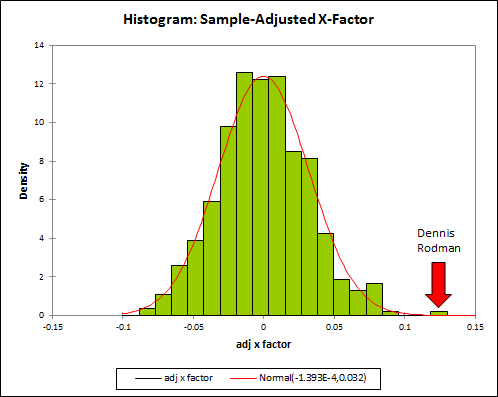
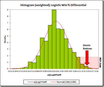
It is common to hear analysts and researchers refer to the p-value as the probability that an outcome occurred by chance. This is called the Odds-Against-Chance Fallacy [60]. One example of the fallacy occurred in a 2011 post about former NBA basketball player Dennis Rodman on the blog Skeptical Sports, analyst Benjamin Morris, now with FiveThirtyEight, wrote that, “The many histograms…reflect fantastic p-values (probability that the outcome occurred by chance) for Dennis Rodman’s win percentage differentials…” But, in fact, the p-value is not the probability that the outcome occurred by chance.
However, as philosophy of science professor Deborah Mayo has pointed out, it may be that some researchers or analysts are simply using this “chance alone” language as a shorthand in normal English speaking, or they might be using an error-probability interpretation of the p-value [7]. In her view not all “chance alone” statements are necessarily incorrect since the researcher may not literally mean the p-value is the probability that the null hypothesis occurred by chance alone. Mayo argues that a more generous approach should be taken and interpretations of “chance alone” statements should be based on what the researcher is actually trying to communicate to the reader or listener.
Of course, it can often be difficult to determine the extent to which an individual citation of the “chance alone” fallacy is simply shorthand or an error-probability interpretation rather than a true misinterpretation on the part of the researcher. Likewise, even academic researchers struggle with p-value interpretations (see fallacies later in this list), so it’s a tall proposition to expect non-academic analysts to understand the subtleties of any “chance alone” statements outside of their literal meaning.
Ruma Falk and Charles Greenbaum trace the confusion back to the language used when talking about “chance alone,” noting that it produces ambiguous conditional probabilities [8]:
Researchers often refer to the p-value of a statistical test as “the probability that the results are due to chance.” This phrase is quite slippery. It can be interpreted as “the conditional probability of chance, given the results,” as well as “the conditional probability of the results, given chance.”
However, only the latter of the two statements is correct.
What’s more, Falk and Greenbaums’s reference to the interpretation of the p-value as “the probability that the results are due to chance” is only one of many variations. Benjamin Morris’s language mentioned at the opening of this section was slightly different, the p-value was defined as the “probability that the outcome occurred by chance.” So too is the language used in the title of this fallacy that the p-value is “the probability that chance alone produced the result,” a phrase noted in Greenland et al.’s 2016 article on common statistical misinterpretations [3]. All of these “chance alone” statements are incorrect if understood literally, the p-value is a probability computed assuming chance is operating alone .
Further ambiguity is added by usage of the word “chance,” which may be unclear to those without more rigorous exposure to p-values. In this context the word “chance” refers specifically to random sampling error.
There are undoubtedly some researchers and analysts who have a clear understanding of p-values and nonetheless use various shorthand language which includes statements about “chance alone.” Strictly speaking, however, any “chance alone” statements are incorrect when implicitly or explicitly referencing the probability of the null hypothesis. All things considered, it is probably best to avoid confusion with imprecise “chance alone” statements, even in shorthand.
Fallacy 3: A non-significant p-value indicates no effect between the treatment and control
This mistaken understanding is called the Nullification Fallacy [61]. This fallacy is one of the bases for the current interpretation of statistical significance, a concept not supported by many statisticians [9]. A statistically nonsignificant result — typically defined as a p-value greater than 0.05 — simply indicates that the data are not unusual under the assumptions of the model. These assumptions include that the null hypothesis is true and that only random error is operating on the data.
It’s important to remember that:
Only a p-value of 1 indicates the null hypothesis is the hypothesis most compatible with the data. However, even in this case many other hypotheses are also consistent with the data and a p-value of 1 does not prove the null is true. A determination of no difference between groups cannot be made from a p-value, regardless of size [10].
The observed point estimate for a given experiment is always the effect size most compatible with the data, regardless of the statistical significance [11]. This means that unless the effect size is zero — an estimate of no difference between groups — then the null hypothesis is not the hypothesis most compatible with the data (the null hypothesis does not have to be defined as no difference between groups, but in A/B testing and many other applications no difference is the most common null).
The p-value represents a tail probability and so includes observations that are larger than the observed outcome. For example, a p-value of 0.3 means that, assuming the null hypothesis is true, the observed outcome — and observations more extreme — would be seen 30% of the time (if only random error were operating on the data) [12, 13]. This “more extreme” interpretation can initially be unintuitive. Marketing professor Raymond Hubbard and accounting professor Murray Lindsay have a nice explanation in their paper, “Why P Values Are Not a Useful Measure of Evidence in Statistical Significance Testing” [14]. Hubbard and Lindsay use a famous statistical example known as The Lady Tasting Tea to show why more extreme values are required in the interpretation of p-values.
The p-value assumes that only random error is operating on the data. There are many known violations of this assumption in many business scenarios. For example, in A/B website testing systematic error could arise from:
Users blocking cookies
Slow internet connections causing A/B testing software to time out
Inconsistent implementation of web telemetry between treatment and control
Malfunctioning A/B testing software
A/B testing software that was incorrectly implemented
Changes to the website being introduced while the test is live (a so-called website “refresh”)
Fallacy 3 is extremely common, even among PhD researchers [15]. Several surveys of previous literature have examined the percentage of journal articles in which the authors equated a nonsignificant p-value with evidence of no effect. This research is summarized in the table below. Note that this survey research does not attempt to address what the article authors actually understand about null hypothesis significance testing. It may be that the authors are simply using imprecise language in their articles. Nonetheless, regardless of their understanding the authors were judged on the written p-value interpretations used in their journal articles.
| Survey | Time period | Number of articles examined | Percentage of articles with errors | Definition of "error" |
|---|---|---|---|---|
| Schatz P, Jay KA, McComb J, McLaughlin JR (2005). Misuse of statistical tests in Archives of Clinical Neuropsychology publications. Archives of Clinical Neuropsychology 20:1053-1059 | 2001-2004 | 170 | 48% (81 articles) | “using statistical tests to confirm the null, that there is no difference between groups” | Fidler F, Burgman MA, Cumming G, Buttrose R, Thomason N. (2006). Impact of criticism of null hypothesis significance testing on statistical reporting practices in conservation biology. Conservation Biology 20:1539-1544 | 2005 | 100 | 42% (42 articles) | “statistically nonsignificant results were interpreted as evidence of ‘no effect’ or ‘no relationship'" | Hoekstra R, Finch S, Kiers HAL, Johnson A. (2006). Probability as certainty: dichotomous thinking and the misuse of p values. Psychonomic Bulletin & Review 13:1033 1037 | 2002-2004 | 259 | 56% (145 articles) | “Phrases such as ‘there is no effect,’ ‘there was no evidence for’ (combined with an effect in the expected direction), ‘the nonexistence of the effect,’ ‘no effect was found,’ ‘are equally affected,’ ‘there was no main effect,’ ‘A and B did not differ,’ or ‘the significance test reveals that there is no difference’" | Bernardi F, Chakhaia L, Leopold L. (2017). ‘Sing me a song with social significance’: the (mis)use of statistical significance testing in European sociological research. European Sociological Review 33:1-15 | 2010-2014 | 262 | 51% (134 articles) | “authors mechanically equate a statistically insignificant effect with a zero effect” |
Fallacy 4: A statistically significant p-value indicates the null hypothesis is false
This is the inverse of Fallacy 3. A statistically significant result — typically defined as a p-value less than 0.05 — simply indicates the data are unusual under the assumptions of the model.
It’s important to remember that:
A key assumption of NHST calculations is that the null hypothesis is true. A small p-value simply indicates that the observed data are not very compatible with the null hypothesis. This can happen for three reasons:
The null hypothesis is false.
A large random sampling error was observed in the data.
The model was incorrectly specified, for example it did not account for non-random error present in the data collection process (see Item 6 below).
Even if a small p-value was generated because the null hypothesis is false this does not always have practical importance. For instance, if the null hypothesis is defined as no difference between group means, as is often the case, there could be effect sizes that are non-zero, but practically unimportant to the problem at hand.
The NHST framework does not use observed data to test the compatibility of the null hypothesis relative to the alternative hypothesis.
Statistical significance is an interpretation of the result of a test, not of the phenomenon being studied. It is therefore not correct to say that one has found “evidence of” a statistically significance effect. There is either no effect or some effect, quantified by a point estimate and corresponding confidence interval. A p-value threshold does not produce evidence [13]. Some statisticians do interpret the p-value itself as a measure of evidence to the extent that it measures the compatibility of the null hypothesis with the observed data.
Statistically significant p-values can have high false positive risk [6].
The p-value can be sensitive to random errors in the data. These random errors can easily cause a p-value to cross the statistical significance threshold (see our article on p-value replicability for details). In addition, non-random errors will affect the p-value if they are present in the data generating process and not explicitly accounted for in the model. For example, in A/B website testing systematic error could arise from:
Users blocking cookies
Slow internet connections causing A/B testing software to time out
Inconsistent implementation of web telemetry between treatment and control
Malfunctioning A/B testing software
A/B testing software that was incorrectly implemented
Changes to the website being tested while the test is live (a so-called website “refresh”)
Fallacy 5: The size of the p-value represents the strength of the treatment
The p-value is sometimes interpreted as an effect size, with smaller p-values indicating more of an effect. This is called the Effect Size Fallacy [60]. In a 1979 study Michael Oakes set out to study the Effect Size Fallacy and found that psychology researchers overestimated the size of the effect when the significance threshold was changed from 0.05 to 0.01. Oakes asked 30 academic psychologists to answer the prompt below [16]:
Suppose 250 psychologist and 250 psychiatrists are given a test of psychopathic tendencies. The resultant scores are analysed by and independent means t-test which reveals that the psychologists are significantly more psychopathic than the psychiatrists at exactly the 0.05 level of significance (two-tailed) If the 500 scores were to be rank ordered, how many of the top 250 (the more psychopathic half) would you guess to have been generated by psychologists?
| Significance level | ||
|---|---|---|
| 0.05 | 0.01 | |
| 0.05 level presented first | 163 | 181 |
| 0.05 level presented second | 163 | 184 |
Table notes:
1. Sample sizes: academic psychologists first presented 0.05 and then asked to revise at 0.01 (n=30); academic psychologists first presented 0.01 and then asked to revise at 0.05 (n=30).
2. The standard deviation for all four groups was around 20, ranging from 18.7 to 21.2.
3. Reproduced from Michael Oakes, Statistical Inference, Epidemiology Resources Inc. [link]; the book was published in 1990, but the study was conducted in 1979.
The participants were then asked to revise their answer assuming the 0.05 level of significance was changed to 0.01. For a separate set of an additional 30 academic psychologists the order of the prompts was reversed, with respondents asked first about the 0.01 level and then about the 0.05 level.
The results of the respondents’ answers are shown in the table at right (answers have been rounded). The first row shows responses from the group asked first to consider the 0.05 significance level while the second row shows responses from the group asked first to consider the 0.01 significance level.
The correct answer is that moving from a level of significance of 0.05 to a level of 0.01 implies three additional psychologists appear in the top 250. However, the average answers for both groups shows that on average the psychologists estimated a difference of around 20 additional psychologists would appear in the top 250. Oakes also calculated the median responses, which did not substantively change the results.
Andrew Gelman and Hal Stern report a more recent case of researchers making the same mistake [17]. The authors examined a study in which researchers attempted to measure the health effects of low-frequency electromagnetic fields. The researchers modulated the electromagnetic fields to different frequencies and measured the effect on the functioning of chick brains. Different frequencies achieved different levels of statistical significance. Gelman and Stern note:
The researchers used this sort of display to hypothesize that one process was occurring at 255, 285, and 315 Hz (where effects were highly significant), another at 135 and 225 Hz (where effects were only moderately significant), and so forth…
The researchers in the chick-brain experiment made the common mistake of using statistical significance as a criterion for separating the estimates of different effects, an approach that does not make sense.
Authors Jeffrey Gliner, Nancy Leech and George Morgan hypothesize that this fallacy is common because of the relationship between p-values and effect sizes [18]. It is indeed true that in general smaller p-values are associated with larger effect sizes (holding sample size and random error constant). For instance, in Oakes’ study a p-value of 0.01 corresponded to 3 additional psychologists in the top 250 compared to a p-value of 0.05. The relationship between p-values and effect sizes was part of our explanation about NHST and one of the reasons for the zone of nonsignificance. Indeed, because p-values are designed to exhibit natural variation due to random error, the relationship between p-values and their associated effect sizes appears to be weaker than many realize [19].
Oakes also notes that, “[I]t is with large samples that the disparity between statistical significance and effect size is most marked” [16]. This is because larger sample sizes allow the detection of very small differences between groups and so it doesn’t take much of a change in the estimated effect size to influence the p-value. Just such a large sample size example can be seen using web page click-through rate (CTR). Imagine an A/B test with sample sizes of 53-thousand for both the treatment and control (for a total of 106-thousand) and a baseline CTR of 3.0% (this experimental setup was designed to give a power of 80% to detect a lift of 10% — from 3.0% to 3.3% — with a Type I error rate of 5%). The difference between a CTR of 3% and 3.3% produces a highly significant p-value of 0.005. Reduce the CTR by just a tenth of a percent to 3.2% and the p-value is an order of magnitude larger, 0.05. Reduce CTR by another tenth of a percent to 3.1% and the p-value becomes 0.34.
The bottom line is that the p-value is not a direct measure of the strength of the treatment. Fallacy 8 (below) demonstrates that two experimental results can have drastically different p-values, but the same effect size because the width of the associated confidence intervals can vary. Fallacy 9 (below) demonstrates the opposite: that two experimental results can have the same p-value, but drastically different effect sizes, again because the confidence interval can vary. The width of the confidence interval itself varies due to variations in random error and sample size.
Fallacy 6: The p-value represents the probability of replication
A common misinterpretation of the p-value is that one minus the p-value describes the probability of replication. This is called the Replication Fallacy [60] or what Gred Gigerenzer calls the “replication delusion” [20]. Under this mistaken paradigm a p-value of 0.05 means there is a 95% chance a repeated experiment would also produce a statistically significant p-value.
Even if one does not strictly believe the replication delusion, many analysts believe a small p-value is somehow indicative of strong replication probabilities, with repeated experiments of an initially statistically significant result likely to produce more statistically significant results most of the time. This is not true.
In his book Statistical Inference, researcher Michael Oakes suggested that misconceptions about replicability might be tied to deeper misconceptions about statistical significance more generally [16]. If one believes that statistical significance is a threshold separating effects that exist (statistically significant results) from effects which do not exist (statistically nonsignificant results) then one likely believes that statistically significant results will replicate since the underlying population difference generating the significant result is “real” and would be detected in follow-up experiments. However, as mentioned in Fallacy 4 above, statistical significance is an interpretation of the result of a statistical test, not of the underlying phenomenon being studied.
In fact, if there is a true difference between the treatment and control -- in other words if the alternative hypothesis is true -- it is the power of the experiment, not the p-value, that tells us the long-term frequency of obtaining statistically significant results upon replication. On the other hand, if the null hypothesis is true then by definition a statistically significant p-value would be seen 5% of the time under normal test setup (with a 5% level set as the Type I error rate).
It can be shown that if an experiment obtained a p-value of 0.05 then a replication of that experiment with equal sample size has only a 50% chance of obtaining a statistically significant p-value [64] (using reasonable assumptions, for example, that the effect size found in the first experiment equals the true, but unknown effect size).
The lack of p-value replication is a natural result of the p-value definition. P-values are meant to be sensitive to normal random fluctuations in data. Even if an experiment is repeated exactly random error can cause the p-value to vary by several orders of magnitude. P-value replication is discussed at length in our article “A/B Testing and p-values: The Subtleties of replication.”
Oakes tested academic psychologists’ understanding of p-values and replication by asking 54 of them to predict via intuition (or direct calculation if desired) the probability of replication under three different scenarios [16].
Suppose you are interested in training subjects on a task and predict an improvement over a previously determined control mean. Suppose the results is Z = 2.33 (p = 0.01, one-tailed), N=40. This experiment is theoretically important and you decide to repeat it with 20 new subjects. What do you think the probability is that these 20 subjects, taken by themselves, will yield a one-tailed significant result at the p < 0.05 level?
Suppose you are interested in training subjects on a task and predict an improvement over a previously determined control mean. Suppose the result is Z = 1.16 (p=0.12, one-tailed), N=20. This experiment is theoretically important and you decide to repeat it with 40 new subjects. What do you think the probability is that these 40 new subjects, taken by themselves, will yield a one-tailed significant result at the p < 0.05 level?
Suppose you are interested in training subjects on a task and predict an improvement over a previously determined control mean. Suppose the result is Z = 1.64 (p=0.05, one-tailed), N=20. This experiment is theoretically important and you decide to repeat it with 40 new subjects. What do you think the probability is that these 40 new subjects, taken by themselves, will yield a one-tailed significant result at the p < 0.01 level?
| Scenario | Mean intuition of replicability | True replicability |
|---|---|---|
| 1 | 80% | 50% |
| 2 | 29% | 50% |
| 3 | 75% | 50% |
Table notes:
1. Reproduced from Michael Oakes, Statistical Inference, Epidemiology Resources Inc. [link]; the book was published in 1990, but the study was conducted in 1979.
The results of Oakes’ test is presented in the table at right. Oakes designed the scenarios in a clever manner so that each of the three scenarios produced the same answer: the true replicability is always 50%. In all three cases the the difference between the average intuition about the replicability of the scenarios and the true replicability is substantial. As outlined above Oakes argues that this difference is due to statistical power being under appreciated by psychologists who instead rely on mistaken notions of replicability linked to the statistical significance of the p-value.
Although Oakes offered “direct calculation if desired” he notes that few participants actually attempted this. It is important to understand that direct calculation of the answers to these questions requires assumptions. For instance, one must assume the effect size calculated from the first sample of subjects in each question is the true effect size. One then needs to use this effect size to calculate the statistical power using the second sample of subjects. Oakes does not discuss the fact that these assumptions are omitted from his questions and does not note any participants bringing up this assumption when discussing his debrief with the participants.
Gerd Gigerenzer undertook a more systematic review of previous studies to understand the depth of the “replication delusion” among academic psychologists and other researchers [20]. His results are reproduced in the table below and show that substantial percentages of the respondents fell prey to the delusion.
| Study | Description of group | Country | N | Statistic tested | Respondents exhibiting the replication delusion |
|---|---|---|---|---|---|
| Oakes (1986) | Academic psychologists | United Kingdom | 70 | p = 0.01 | 60% |
| Haller & Krauss (2002) | Statistics teachers in psychology | Germany | 30 | p = 0.01 | 37% |
| Haller & Krauss (2002) | Professors of psychology | Germany | 39 | p = 0.01 | 49% |
| Badenes-Ribera, Frias-Navarro, Monterde-i-Bort, & Pascual-Soler (2015) | Academic psychologists: personality, evaluation, psychological treatments | Spain | 98 | p = 0.001 | 35% |
| Badenes-Ribera et al. (2015) | Academic psychologists: methodology | Spain | 47 | p = 0.001 | 16% |
| Badenes-Ribera et al. (2015) | Academic psychologists: basic psychology | Spain | 56 | p = 0.001 | 36% |
| Badenes-Ribera et al. (2015) | Academic psychologists: social psychology | Spain | 74 | p = 0.001 | 39% |
| Badenes-Ribera et al. (2015) | Academic psychologists: psychobiology | Spain | 29 | p = 0.001 | 28% |
| Badenes-Ribera et al. (2015) | Academic psychologists: developmental and educational psychology | Spain | 94 | p = 0.001 | 46% |
| Badenes-Ribera, Frias-Navarro, Iotti, Bonilla-Campos, & Longobardi (2016) | Academic psychologists: methodology | Italy, Chile | 18 | p = 0.001 | 6% |
| Badenes-Ribera et al. (2016) | Academic psychologists: other areas | Italy, Chile | 146 | p = 0.001 | 13% |
| Hoekstra, Morey, Rouder, & Wagenmakers (2014) | Researchers in psychology (Ph.D. students and faculty) | Netherlands | 118 | 95% CI | 58% |
Table notes:
1. Reproduced from Gerd Gigerenzer, "Statistical Rituals: The Replication Delusion and How We Got There", Advances in Methods and Practices in Psychological Science, 2018 [link]
Fallacy 7: If the alternative hypothesis is true the p-value will always be small
| Lift | Power | Percent significant | Max p-value | Min p-value |
|---|---|---|---|---|
| 0% | 5% | 10% | 0.79 | 0.03 |
| 5% | 29% | 30% | 0.72 | 0.001 |
| 10% | 80% | 70% | 0.94 | 0.00025 |
| 15% | 98% | 100% | 0.023 | 0.00000008 |
| 20% | 100% | 100% | 0.00005 | 0.0 |
This fallacy is closely related to Fallacy 6. P-values exhibit large natural variation due to random sampling error. Even when the null hypothesis is false this random error can cause the p-value to exhibit large variation even if an experiment is repeated. The table at right shows the p-value range for just 10 simulated A/B tests per row. The experimental setup is simulating an A/B test to assess the impact of a new CTA (the treatment) based on its lift in CTR over the existing CTA (control). The baseline CTR of the control was set to be 3.0%. The sample size was set to detect a true population lift of 10% (from 3.0% CTR to 3.3% CTR) at 80% power with 95% confidence. These specifications led to a sample size of 53,210 customers for both the control and the treatment, for a total of 106,420 customers. Although the sample size was based on the assumption of 10% lift, the true population lift of the treatment CTA varied from 0% to 20% in 5% increments.
Even for the case where the effect of the CTA for the population was exactly the lift chosen to calculate our sample size (10% lift), the p-value ranged from 0.00025 to 0.94 due to random error alone. Again, the large ranges in p-values above are based on just 10 simulated A/B tests! This comes as a surprise to many. If a single experiment produced a statistically significant result at the 0.00025 level, one typically wouldn’t expect a replication of the experiment to produce a p-value of 0.94. This shows that even when the alternative hypothesis is true and the experiment is properly powered, random sampling error can cause the p-value to vary from large to small.
It is important to note that these results are from a particular set of 10 simulated A/B tests. Repeating this simulation again would lead to different results. However, the underlying phenomenon of widely varying p-values would be observed with any set of 10 simulations. Also of note is that because of the limited number of trials in this simulation the percent of statistically significant trials does not match the true power exactly.
P-value variation is discussed at length in our article “A/B Testing and p-values: The subtleties of replication.”
Fallacy 8: Significant and nonsignificant results are contradictory
When examining the results of two different experiments or analyses one might believe that if one experimental result achieved statistical significance while the other did not the two results are somehow in conflict. However, this isn’t necessarily the case. Studies can have different p-values even when the estimated effect size is the same. A conceptual example is given in the chart at right. The two experiments both resulted in an effect size of 10% increase in some theoretical benefit (for example CTR lift). However the p-value of the first is just 0.3 (nonsignificant) while the p-value of the second is 0.002 (highly significant) [21].
As a basic rule of thumb, if the confidence intervals from two experiments overlap it is not correct to say the results conflict. This is because confidence intervals represent values that are compatible with the data that produced them. Therefore, if two confidence intervals overlap it indicates that there is some range of estimated effects which both studies show are compatible with the data.
However, this is just a rule of thumb. Sometimes studies with small ranges of overlapping confidence intervals do have a meaningful difference between estimates. A mathematical analysis can be conducted using a so-called analysis of heterogeneity to more formally determine whether two results conflict [22]. Analysis of heterogeneity produces what is called “I-squared,” a parameter that describes the percentage of total variation across studies that is due to heterogeneity rather than random error. The I-squared calculation can also produces confidence intervals so that qualitative judgement can be used to assess the heterogeneity between studies. Researchers are also coming up with additional methods of conducting meta-analyses, combinations of previous study results into a single coherent whole [23].
Another factor to consider is what “contradictory” or “supportive” means in a particular setting. Two or more experimental results that have an effect size in the same direction — even if the confidence intervals are far from overlapping — could be considered supportive if the question is simply, “Do the studies show the treatment has a positive effect?” However, if a more precise question is considered, for example, “Is the treatment effect of magnitude X,” the results might be considered contradictory.
So to rephrase this fallacy into a correct statement: statistically significant and nonsignificant results are not necessarily contradictory.
Fallacy 9: Studies with the same p-value provide the same evidence against the null hypothesis
This is the inverse of Fallacy 8 and again wrong, however this fallacy is more subtle. To demonstrate consider the chart at right. The two experimental results both have a p-value of 0.05, indicating statistical significance. However, two experiments have different estimated effect sizes of the percent increase in some theoretical benefit (for example CTR lift); the first experiment resulted in an estimated benefit of 19% while the second resulted in an estimated benefit of 3% [24].
The two confidence intervals overlap, so in some sense the results are in fact supportive. Again, a formal analysis would be needed to determine that.
But when taken in the full context there are additional considerations. For instance, the threshold for practical significance must also be considered. If a percent benefit of 10% is required to offset implementation costs then these two results are in conflict: the result with 19% benefit meets the cost-benefit tradeoff while the result with a 3% benefit does not. If these results came from two replications of the same experiment it would be unclear from this information alone whether the treatment should be implemented since one experiment showed the cost-benefit threshold was met and its replication showed it was not.
So to rephrase this fallacy into a correct statement: two or more results with the same p-value do not necessarily provide similar evidence against the null hypothesis.
Fallacy 10: Multiple comparisons are straightforward to adjust for
The general idea of multiple comparisons is fairly well-known to many business analysts. Under standard setups there is a 5% chance that a true null hypothesis will result in a statistically significant p-value. However, if the chance of this kind of error is only 5% with a single test, the chance of this kind of error by any test necessarily increases as the number of tests of significance conducted increases (this is known as the family wise error rate, or FWER). For example, consider a single experiment where multiple success metrics are examined. If, say, 10 different statistical tests are run the FWER increases to 40% (1 - [1 - 0.05]^10 = .40), assuming the 10 metrics are independent.
Because this phenomenon is already accounted for by many business analysts and data scientists doing tests of statistical significance it may lead to the mistaken belief that multiple comparisons is a “solved problem.” There are numerous subtleties to multiple comparisons, however.
One trap goes by what statistician Andrew Gelman calls, “The Garden of the Forking Paths” [25]. To understand the problem let's consider a thought experiment. Suppose you run an A/B test with a new, more prominent “add to cart” button on some product pages. You initially plan on testing the click-through-rate (CTR) on the “add to cart” product pages you have today and comparing it to the version with the improved button. After the test is complete a colleague tells you that there was a small uptick in total sales during the period the test was active. Could the increase be due to the new button? Everyone agrees that based on the data you should abandon the original success metric of CTR and instead conduct the test of statistical significance on the comparison of average order value between the two groups exposed to the differing “add to cart” buttons.
Here’s a question: you ran a single test of statistical significance, do multiple comparisons matter? The surprising answer is yes. Why? Because while you conducted a single test of significance, the choice to run that test was based on first examining the data. Had the data come out differently — perhaps sales saw no uptick — you would’ve stuck with the original plan of evaluating success based on CTR. Different patterns discovered while examining the data would have led to different definitions of success. “[I]f you accept the concept of the p-value, you have to respect the legitimacy of modeling what would have been done under alternative data,” Andrew Gelman and Eric Loken wrote in their 2013 paper on the subject [25].
Pre-examining the data in this way before conducting tests of statistical significance leads to an unconstrained multiple comparisons problem, from which there is no easy way to recover. It’s not possible to adjust for the comparisons in the usual manner because it’s unclear how many comparisons there are to adjust for. Different patterns in the data would’ve lead to an untold number of possible tests of significance. This is what Gelman and Loken mean by “forking paths.” Note that the problem is distinct from the phenomenon of “p-hacking,” intentionally conducting many tests of statistical significance until one of them produces a significant result.
The typical way to address the Garden of the Forking Paths is to separate exploratory analysis and experimentation. Step one is to conduct free form analysis, looking for patterns you may find meaningful. Step two is to fix the success metrics discovered in step one and conduct a careful experiment. However, the Garden of the Forking Paths is just one of dozens of so-called “Researcher Degrees of Freedom,” flexibility that researchers have in formulating hypotheses, and in designing, running, analyzing, and reporting of research [62, 63].
Another challenge is figuring out exactly how one defines a “family” as part of the family-wise error rate [26]. This includes understanding whether there are multiple hypotheses and a single outcome variable (a family of hypotheses), a single hypothesis with multiple outcome variables (a family of outcomes), or some combination of the two.
For example, suppose a data scientist, Alice, who works at an online clothing retail chain, is attempting to classify customers. She is comparing the results of two classification algorithms, a support vector machine and a random forest [27]:
Alice designs a study to compare the performance of a support vector machine with random forest on a particular data set. She carries out her experiments in the morning and observes that the support vector machine performs significantly better than random forest. No corrections for multiple testing are needed because there are just two classifiers. Out of curiosity, Alice then applies naive Bayes to the same data in the evening. Clearly, Alice’s new experiment has no effect on her earlier experiments, but should she make multiplicity adjustments?
Again, pre-specifying outcomes and delineating exploratory and confirmatory analysis can help. But as any analyst knows, that is easier said than done.
Multiple comparisons also get fuzzy at large companies with common use data lakes. Multiple teams may independently “dip” into the lake, running statistical hypothesis tests without awareness that other teams are running separate hypothesis tests on the same subset of data. And what about a series of, say, five A/B web tests run over a period of three months that all target the same set of customers. Should this be thought of as five separate tests with no need for multiplicity adjustments or as a family of five tests requiring adjustment?
Methods to control FWER have been criticized because they need to protect against the most extreme scenario, the so-called “universal null hypothesis,” described by prominent statistician Kenneth Rothman [28]:
The formal premise for such adjustments is the much broader hypothesis that there is no association between any pair of variables under observation, and that only purely random processes govern the variability of all the observations in hand. Stated simply, this “universal” null hypothesis presumes that all associations that we observe (in a given body of data) reflect only random variation.
But Rothman notes that:
For the large bodies of data for which adjustments for multiple comparisons are most enthusiastically recommended, the tenability of a universal null hypothesis is most farfetched. In a body of data replete with associations, it may be that some are explained by what we call “chance,” but there is no empirical justification for a hypothesis that all the associations are unpredictable manifestations of random processes. The null hypothesis relating a specific pair of variables may by only a statistical contrivance, but at least it can have a scientific counterpart that might be true. A universal null hypothesis implies not only that variable number six is unrelated to variable number 13 for the data in hand, but also that observed phenomena exhibit a general disconnectivity that contradicts everything we know.
Controlling the FWER under the universal null hypothesis requires a bigger adjustment than if fewer null hypotheses were true and causes a bigger reduction in power. If the universal null is very unlikely to be true, then the multiplicity adjustment may be causing a needless loss of power, or excessive sample sizes to counteract this effect. However, the null of true null hypotheses is generally unknown, in which case the number to adjustment for is not clear.
There are other multiple comparisons methods that focus on a different criterion than the FWER, for instance the false discovery rate (FDR), which attempts to control the expected proportion of false positives. However, FDR has its own drawbacks. Andrew Gleman has noted that FDR may be useful in applications such as genetics where there are expected to be a large number of truly zero interactions. However, according to Gelman FDR, “may be less useful in social science applications when we are less likely to be testing thousands of hypotheses at a time and when there are less likely to be effects that are truly zero.” Most business applications are likely closer to the social science model than the genetics model.
For all of the reasons listed above, statisticians like Rothman and Gelman have suggested that multiple comparisons may not be needed at all in many applications [28, 29]. But multiple comparisons is so thorny that even they are not always resolute in the best approach. In fact, Gelman titled a short 2014 blog post, “In one of life’s horrible ironies, I wrote a paper ‘Why we (usually) don’t have to worry about multiple comparisons’ but now I spend lots of time worrying about multiple comparisons.”
Statisticians Arvid Sjölander and Stijn Vansteelandt highlighted the difficulty of multiple comparisons approaches in their 2019 paper, “[T]he issue of multiplicity adjustment is surrounded by confusion and controversy, and there is no uniform agreement on whether or when adjustment is warranted” [30].
While statisticians Sander Greenland and Albert Hofman disagreed with the methods suggested by Sjölander and Vansteelandt in their paper, they too agree that multiple comparisons is a difficult problem [31]:
Given that even elementary issues like simple statistical testing have engendered no consensus in their 300-year history, how could we expect agreement about more subtle issues? Without consensus on the basics, it should be no surprise that such a complex topic as multiple comparisons is so widely misunderstood and in conflict.
To correct the title of this fallacy, multiple comparisons are not always straightforward to adjust for.
Fallacy 11: A Meta-analysis is better than a single study
Before addressing this fallacy it’s important to distinguish literature reviews and meta-analysis, both methods of combining previous research.
Literature reviews are qualitative readings of a set of academic papers, although the method by which those papers are selected is often rigorous (for example, using a particular set of keywords and then filtering on a pre-defined criteria). Literature reviews are meant to get a sense of the current state of research. What direction are the papers pointing? Are there any conflicting findings? What are the gaps in research that need to be addressed?
Meta-analysis is a statistical method for combining data from multiple papers quantitatively. For example, a new p-value may be calculated by combining results from 10 previous papers, each of which collected its own data and calculated its own p-value. As Brian Haig put it, “By calculating effect sizes across primary studies in a common domain, meta-analysis helps us detect robust empirical generalizations” [32].
When presented with a meta-analysis a naive business analyst or data scientist may interpret the evidence to be especially strong due to the perceived strength of combined studies. Indeed, many researchers would agree that no one study should ever be thought of as definitive. Both literature reviews and meta-analysis have the advantage of looking at multiple studies. For this reason it has been noted that, “meta-analysis is thought by many to be the platinum standard of evidence” [33]. No wonder meta-analyses are on the rise [34] with more than 11,000 published in 2018 [35].
There are a few problems with the “platinum standard” view, however. One is that meta-analyses are only as good as the studies they are synthesizing. A recent example of this fact was demonstrated in research connecting depression to the transporter gene 5-HTTLPR. Consider the following passage describing various linkages found involving 5-HTTLPR [36]:
A meta-analysis of twelve studies found a role (p = 0.001) in PTSD. A meta-analysis of twenty-three studies found a role (p = 0.000016) in anxiety-related personality traits...A meta-analysis looked at 54 studies of the interaction and found “strong evidence that 5-HTTLPR moderates the relationship between stress and depression...A meta-analysis of 15 studies found that 5-HTTLPR genotype really did affect SSRI efficacy (p = 0.0001)…
All of those meta-analyses turned out to be incorrect and did not replicate in better designed studies with much larger sample sizes [37, 38]. There are numerous other examples of meta-analyses being overturned (see for example 39, 40, and 41).
One reason for this is that journals have a tendency to only publish findings with statistically significant results, and so the current body of research from which meta-analyses can draw isn’t representative of all findings [42]. (Publication bias is sometimes known as the file-drawer problem, so-called because non-significant findings are never published and instead go in the file drawer).
The product of publication bias was highlighted in a December 2019 study appearing in Nature Human Behavior in which researchers compared 15 psychology meta-analyses to comparable multi-laboratory replications. The researchers found on average that meta-analysis effect sizes are overstated almost three times [43].
Don’t forget that research is hard! There are many ways research can go wrong including nefarious or inadvertent p-hacking or simply poor research design or analysis. Meta-analyses have the additional difficulty of attempting to combine multiple, disparate studies into a single coherent whole. A 2007 study reviewed 27 meta-analyses that had employed the standardized mean differences (SMD) approach used to synthesize multiple studies that used different measurement scales. The analysis found that 17 (63%) of the meta-analyses contained errors [44]. But many other journal articles have pointed out the subtleties in combining multiple studies. For example, the correct statistical techniques to use in randomized binomial trials with low event rates [45], subgroup variance analysis methods [46], and proper subjective coding and decision rules [47].
The criteria by which studies are chosen for presentation in a meta-analysis introduces human bias and subjectivity; so do other aspects of meta-analysis preparation like data extraction from the preexisting research [48]. Even the act of searching for articles for inclusion in meta-analysis requires human judgement [48].
As one paper, titled “Meta-analysis: pitfalls and hints,” put it [49]:
Meta-analysis is a powerful tool to cumulate and summarize the knowledge in a research field, and to identify the overall measure of a treatment’s effect by combining several conclusions. However, it is a controversial tool, because even small violations of certain rules can lead to misleading conclusions. In fact, several decisions made when designing and performing a meta-analysis require personal judgment and expertise, thus creating personal biases or expectations that may influence the result.
The result is that different meta-analysis on the same topic can conflict [50]. One example of conflicting findings is shown on the insert at right, which was reproduced from a 2018 Science Magazine article by Jop de Vrieze [35]. Two meta-analyses created just one year apart attempted to examine whether the health response of taking a placebo was increasing over time. The two studies took different approaches to the types of studies used for inclusion in the analysis, the outcome measures, and the statistical methods. As a result the two studies reached different conclusions.
But that is far from the only case of conflicting meta-analyses. Consider, for instance, the so-called “worm wars,” conflicting findings involving the deworming of children in low-income countries [51]. Such deworming campaigns became popular under the recommendation of the World Health Organization (WHO). In 2015 a meta-analysis found that deworming was primarily ineffective, noting that [52]:
[I]n mass treatment of all children in endemic areas, there is now substantial evidence that this does not improve average nutritional status, haemoglobin, cognition, school performance, or survival.
But a second meta-analysis by different authors one year later found that deworming was quite efficient at improving nutrition [53]:
[T]he estimated average weight gain per dollar is more than 35 times that from school feeding programs…
Similar conflicts were seen in meta-analyses examining the impact of violent video games and media coverage on real-world aggression. A 2009 study was published in the Journal of Pediatrics which found, “[L]ittle support for the hypothesis that media violence is associated with higher aggression” [54].
However, just one year later a second group of researchers released a contradictory meta-analysis in which the authors criticized the design of the previous study, noting for example that their revised research used, “more restrictive methodological quality inclusion criteria than in past meta-analyses” and finding that overall, “The evidence strongly suggests that exposure to violent video games is a causal risk factor for increased aggressive behavior, aggressive cognition, and aggressive affect and for decreased empathy and prosocial behavior” [55]. To make things even more exciting a third article was released in 2010 arguing that the methodologies of the second meta-analysis were themselves flawed and the original 2009 paper was mostly correct. The authors of the 2010 paper concluded that, “[T]he effects of violent games on aggressive behavior in experimental research are estimated as being very small…” [56].
This was not the end of the story, however. A paper titled, “Finding Common Ground in Meta-Analysis “Wars” on Violent Video Games” was released in 2019 that attempted to resolve the disputes between these and other conflicting meta-analyses [71]. The paper claimed that the difference in findings of the previous studies were actually the result of the analytical approaches employed and that better statistical methods could show the studies were actually in agreement. As the article’s title suggests, it found the “common ground” that, “the vast majority of settings, violent video games do increase aggressive behavior but that these effects are almost always quite small.”
No wonder the aforementioned article in Science Magazine was titled, “Meta-analyses were supposed to end scientific debates. Often, they only cause more controversy.” Jacob Stegenga echoed the difficulties involved when combining multiple studies into a meta-analysis in his paper, “Is meta-analysis the platinum standard of evidence?” noting that there are many analytic decisions that have to be made when combining previous research [33]:
I argue that meta-analysis falls far short of [the platinum] standard. Different meta-analyses of the same evidence can reach contradictory conclusions. Meta-analysis fails to provide objective grounds for intersubjective assessments of hypotheses because numerous decisions must be made when performing a meta-analysis which allow wide latitude for subjective idiosyncrasies to influence its outcome.
A related problem is that meta-analyses don’t always generalize. Here the word “generalize” follows the normal definition used in casual English. It means that the observed phenomenon is real and applies in a variety of contexts (i.e. that it is not merely an artifact of the specific subpopulation examined in the study). In their article, “Meta-Analysis and the Myth of Generalizability” researchers Robert Tett, Nathan Hundley, and Neil Christiansen examined 24 meta-analytical articles that used a total of 741 aggregations of previously reported data [72]. “In support of the noted concerns, only 4.6% of the 741 aggregations met defensibly rigorous generalizability standards,” the authors wrote.
Metascience specialist John Ioannidis has written that, “Few systematic reviews and meta-analyses are both non-misleading and useful” [34]. Michael Oakes in his book Statistical Inference was even more critical, writing that, “I … regard the recently exhibited enthusiasm for meta-analysis as a retrograde development” [16]. Oaks goes on to criticize three different methods of producing meta-analyses. Oakes’ feelings may be especially harsh, but they speak to the fact that simply throwing together multiple studies does not magically make the whole greater than the sum of its bad parts.
None of this is meant to imply that all meta-analyses are bad. But they are not all good either. The platinum standard of academic research is good research. There is no universal formula for what “good research” means, it varies from study to study and depends on the context. Meta-analyses should be viewed with the same healthy skepticism as any single study. Indeed, just like an individual study many design decisions go into the creation of a meta-analysis and just like an individual study the integrity of the underlying data is paramount to the quality of the final product. (Many of the points made in this fallacy explanation were also made by Geoffrey Kabat in his two-page June 2020 article in Significance, which is a short and accessible read for those interested [65]).
To rephrase this fallacy, a meta-analysis is not necessarily better than an individual study.
Fallacy 12: The calculation of the p-value is independent of experimental design
Many business analysts and data scientists may not be aware that the p-value depends on how a particular experiment is thought about in terms of possible experimental outcomes. One simple example is whether an analyst has chosen to test if the treatment is better than the control (a one-sided test) or testing whether it is better or worse (a two-sided test). The same data considered under one- or two-sided tests will produce different p-values.
But one and two-sided tests are just one example of how design can influence the p-value calculation. Consider the thought experiment below, adapted from Daniel Berrar’s “Confidence curves: an alternative to null hypothesis significance testing for the comparison of classifiers” [57]. (P-value calculations have been omitted, but can be found in the original paper. The hypothetical situations below are based on the famous Lady Tasting Tea thought experiment, of which there is a short but useful treatment in Raymond Hubbard and Murray Lindsay’s paper, “Why P Values Are Not a Useful Measure of Evidence in Statistical Significance Testing” [58]).
Suppose that Alice and Bob work together at a credit agency and have jointly developed a new machine learning classifier NEW-C to help with lending decisions. The classifier will examine customer attributes and classify the customer as either low, medium, or high risk of credit default.
They believe that NEW-C can outperform another classifier ALT-C on a range of customer data sets. Both Alice and Bob formulate the null hypothesis as follows: the probability that NEW-C is better than ALT-C is 0.5. Alice and Bob decide to benchmark their algorithm independently and then compare their results later. Both Alice and Bob select the same set of six customer datasets that are used at the company for benchmarking new lending classifiers.
Alice is determined to carry out all six benchmark experiments, even if her algorithm loses the competition on the very first few data sets. After all six experiments, she notes that NEW-C was better on the first five data sets, but not on the last data set. Under the null hypothesis, Alice obtains 0.11 as the one-sided p-value. Consequently, she concludes that NEW-C is not significantly better than the competing ALT-C.
Bob has a different plan. He decides to stop the benchmarking as soon as NEW-C fails to be superior. Coincidentally, Bob analyzed the data sets in the same order as Alice did. Consequently, Bob obtained the identical benchmark results. But Bob’s calculation of the p-value is different from Alice’s. In Bob’s experiment, the failure can only happen at the end of a sequence of experiments because he planned to stop the benchmarking in case that NEW-C performs worse than ALT-C. Therefore, Bob obtains 0.03 as the one-sided p-value. And he concludes that their new classifier is significantly better than the competing model ALT-C. The conundrum is that both Bob and Alice planned their experiments well. They used the same data sets and the same models, yet their p-values—and in this example, their conclusions—are quite different.
Before Bob continues with his research, he discusses his experimental design with his supervisor, Carlos. Bob plans to compare their algorithm with an established algorithm OLD-C. This time, the null hypothesis is stated as follows: probability that his algorithm performs differently from OLD-C is 0.5. Thus, this time, it is a two-sided test. Bob decides to benchmark his algorithm against OLD-C on ten data sets, testing against all ten even if NEW-C loses to OLD-C on the first few tests. He observes that his algorithm outperforms OLD-C in 9 of 10 data sets. The two-sided p-value is 0.021. Given that the p-value is smaller than 0.05, Bob concludes that his algorithm is significantly better than OLD-C.
Alice discusses a different study design with Carlos. She also wants to investigate the same ten data sets; however, if she cannot find a significant difference after ten experiments, then she wants to investigate another ten data sets. Thus, her study has two stages, where the second stage is merely a contingency plan. Her null hypothesis is the same as Bob’s. She uses again the same data sets as Bob did, and in the same order. Therefore, she also observes that her algorithm outperforms OLD-C in 9 out of 10 data sets. Thus, she does not need her contingency plan.
However, after discussing her result with Carlos, she is disappointed: her two-sided p-value is 0.34. How can that be? After all, she did exactly the same experiments as Bob did and obtained exactly the same results! This is highly counterintuitive, but it follows from the logic of the p-value. After the first 10 experiments, the outcomes that are as extreme as her actually observed results are 1 and 9. The more extreme results are 0 and 10. In the two-stage design, however, the total number of possible experiments is 20. In the words of Berger and Berry, “[T]he nature of p values demands consideration of any intentions, realized or not” [59]. It does not matter that Alice did not carry out her contingency plan. What matters is that she contemplated to do so before obtaining her results, and this does affect the calculation of her p-value. This is similar to the Garden of the Forking Paths discussed in Fallacy 10.
Berrar ends by noting the following:
Even if sufficient evidence against a hypothesis has been accrued, the experiment must adhere to the initial design; otherwise, p values have no valid interpretation. The frequentist paradigm requires that the investigator adhere to everything that has been specified before the study. Realized or not, the intentions of the investigator matter…
The point of Berrar’s thought experiment is that the drawbacks of p-values outweigh their usefulness and p-value functions should be used instead. Regardless of whether one agrees with Berrar on that particular point, it is important to know that the calculation of the p-value is dependent on the experimental setup.
But experimental design at this level is just one of dozens of so-called “Researcher Degrees of Freedom,” flexibility that researchers have in formulating hypotheses, and in designing, running, analyzing, and reporting of research [62, 63]. Multiple studies of this flexibility show that it can impact results of resulting research [66-70].
Fallacy 12 might not be a practical concern for the majority of business analysts since in many applied situations p-values are calculated based on a standardized setup, for instance in A/B web testing where the p-value is calculated by A/B testing software. However, if an analyst wishes to vary the design of this standard setup outside of normal parameters that design may have implications for the calculation of the p-value.
References
Ronald Wasserstein, Allen Schirm, & Nicole Lazar, “Moving to a World Beyond ‘p < 0.05’”, The American Statistician, 2019 [link]
Ronald Fisher, Statistical methods and scientific inference, 1956 [link]
Greenland et. al., “Statistical tests, P values, confidence intervals, and power: a guide to misinterpretations”, European Journal of Epidemiology, 2016 [link]
Charles Lambdin, “Significance tests as sorcery: Science is empirical— significance tests are not”, Theory & Psychology, 2012 [link]
John Allen Paulos, A Mathematician Plays The Stock Market, 2003 [link]
David Colquhoun, “The False Positive Risk: A Proposal Concerning What to Do About P-values”, The American Statistician, 2019 [link]
Deborah Mayo, “‘A small p-value indicates it’s improbable that the results are due to chance alone’ –fallacious or not? (more on the ASA p-value doc)”, Error Statistics Philosophy (blog), 2016 [link]
Ruma Falk and Charles Greenbaum, “Significance Tests Die Hard: The Amazing Persistence of a Probabilistic Misconception”, Theoretical Psychology, 1995 [link]
The Research, “Statisticians hate statistical significance”, 2019 [link]
Greenland et. al., “Statistical tests, P values, confidence intervals, and power: a guide to misinterpretations” (Misinterpretations #4, #5, #6), European Journal of Epidemiology, 2016 [link]
Steven Goodman, “A Dirty Dozen: Twelve P-Value Misconceptions” (Misconception #2), Seminars in Hematology, 2008 [link]
Steven Goodman, “A Dirty Dozen: Twelve P-Value Misconceptions” (Misconception #2) (Introduction), Seminars in Hematology, 2008 [link]
Greenland et. al., “Statistical tests, P values, confidence intervals, and power: a guide to misinterpretations” (Misinterpretations #4, #9), European Journal of Epidemiology, 2016 [link]
Raymond Hubbard and R. Murray Lindsay, “Why P Values Are Not a Useful Measure of Evidence in Statistical Significance Testing”, Theory & Psychology, 2008 [link]
Valentin Amrhein et al., “Supplementary information to: Retire statistical significance”, Nature, 2019 [link]
Michael Oakes, Statistical Inference, Epidemiology Resources Inc., 1990 [link]
Andrew Gelman and Hal Stern, “The Difference Between “Significant” and “Not Significant” is not Itself Statistically Significant”, The American Statistician, 2006 [link]
Jeffrey Gliner, Nancy Leech, and George Morgan, “Problems With Null Hypothesis Significance Testing (NHST): What Do the Textbooks Say?", The Journal of Experimental Education, 2002 [link]
The Research, “A/B testing and p-values: the subtleties of replication”, 2020 [link]
Gerd Gigerenzer, "Statistical Rituals: The Replication Delusion and How We Got There", Advances in Methods and Practices in Psychological Science, 2018 [link]
Steven Goodman, “A Dirty Dozen: Twelve P-Value Misconceptions” (Misconception #4), Seminars in Hematology, 2008 [link]
Julian Higgins, Simon Thompson, Jonathan Deeks, and Douglas Altman, “Measuring inconsistency in meta-analyses”, The BMJ, 2003 [link]
Rachael Meager, “Understanding the Average Impact of Microcredit Expansions: A Bayesian Hierarchical Analysis of Seven Randomized Experiments”, American Economic Journal: Applied Economics, 2019 [link]
Steven Goodman, “A Dirty Dozen: Twelve P-Value Misconceptions” (Misconception #5), Seminars in Hematology, 2008 [link]
Andrew Gelman and Eric Loken, “The garden of forking paths: Why multiple comparisons can be a problem, even when there is no “fishing expedition” or “p-hacking” and the research hypothesis was posited ahead of time”, Unpublished white paper, 2013 [link]
Beasley et. al., “Common scientific and statistical errors in obesity research”, Obesity, 2016 [link]
Dan Nettleton, “Multiple Testing” (Lecture Notes), 2018 [link]
Kenneth Rothman, “No Adjustments are Needed for Multiple Comparisons”, Epidemiology, 1990 [link]
Andrew Gelman, Jennifer Hill, and Masanao Yajima,” Why We (Usually) Don’t Have to Worry About Multiple Comparisons”, Journal of Research on Educational Effectiveness, 2012 [link]
Arvid Sjölander and Stijn Vansteelandt, “Frequentist versus Bayesian approaches to multiple testing”, European Journal of Epidemiology, 2019 [link]
Sander Greenland and Albert Hofman, “Multiple comparisons controversies are about context and costs, not frequentism versus Bayesianism”, European Journal of Epidemiology, 2019 [link]
Brian D. Haig, “The Philosophy of Quantitative Methods”, Oxford handbook of Quantitative Methods, Vol 1, Oxford University Press, 2012 [link]
Jacob Stegenga, “Is meta-analysis the platinum standard of evidence?”, Studies in History and Philosophy of Science, 2011 [link]
John Ioannidis, “The Mass Production of Redundant, Misleading, and Conflicted Systematic Reviews and Meta-analyses”, The Milbank Quarterly, 2016 [link]
Jop de Vrieze, “Meta-analyses were supposed to end scientific debates. Often, they only cause more controversy”, Science Magazine, 2018 [link]
Scott Alexander, “5-HTTLPR: A pointed review”, Slate Star Codex (bog), 2019 [link]; this is a summarized write-up of the paper in the reference below about which one of the original co-authors, Matt Keller, said on Twitter: “I have never in my career read a synopsis of a paper I've (co-)written that is better than the original paper. Until now. I have no clue who this person is or what this blog is about, but this simply nails every aspect of the issue.”
Border et. al., “No Support for Historical Candidate Gene or Candidate Gene-by-Interaction Hypotheses for Major Depression Across Multiple Large Samples”, American Journal Of Psychiatry, 2019 [link]
Robert Culverhouse, Nancy Saccone, and Laura Jean Bierut, “Collaborative meta-analysis finds no evidence of a strong interaction between stress and 5-HTTLPR genotype contributing to the development of depression”, Molecular Psychiatry, 2018 [link]
Jacob Rosenberg & Kristoffer Andresen, “Wrong conclusion in meta-analysis”, Hernia, 2020 [link]
Lock et. al., “When meta-analyses get it wrong: response to ‘treatment outcomes for anorexia nervosa: a systematic review and meta-analysis of randomized controlled trials’”, Psychological Medicine, 2019 [link]
David Allison and Myles Faith, “Hypnosis as an adjunct to cognitive-behavioral psychotherapy for obesity: a meta-analytic reappraisal”, Journal of Consulting and Clinical Psychology, 1996 [link]
Vosgerau et. al., “99% impossible: A valid, or falsifiable, internal meta-analysis”, Journal of Experimental Psychology: General, 2019 [link]
Amanda Kvarven, Eirik Strømland, and Magnus Johannesson, “Comparing meta-analyses and preregistered multiple-laboratory replication projects”, Nature Human Behavior, 2019 [link]
Peter Gøtzsche, Asbjørn Hróbjartsson, Katja Marić, and Britta Tendal, “Data Extraction Errors in Meta-analyses That Use Standardized Mean Differences”, The Journal of the American Medical Association, 2007 [link]
Jonathan Shuster and Michael Walker, “Low-event-rate meta-analyses of clinical trials: implementing good practices”, Statistics in Medicine, 2016 [link]
Rubio-Aparicio et. al., “Analysis of categorical moderators in mixed-effects meta-analysis: Consequences of using pooled versus separate estimates of the residual between-studies variances”, British Journal of Mathematical and Statistical Psychology, 2017 [link]
R. J. Bullock and Daniel Svyantek, “Analyzing meta-analysis: Potential problems, an unsuccessful replication, and evaluation criteria”, Journal of Applied Psychology, 1985 [link]
David Felson, “Bias in meta-analytic research”, Journal of Clinical Epidemiology, 1992 [link]
Greco et. al., “Meta-analysis: pitfalls and hints”, Heart Lung Vessel, 2013 [link]
Anders Jørgensen, Jørgen Hilden, and Peter Gøtzsche, “Cochrane reviews compared with industry supported meta-analyses and other meta-analyses of the same drugs: systematic review”, The BMJ, 2006 [link]
David Evans, “Worm Wars: The Anthology”, World Bank Blogs, 2015 [link]
Taylor‐Robinson et. al., “Deworming drugs for soil‐transmitted intestinal worms in children: effects on nutritional indicators, haemoglobin, and school performance”, Cochrane Systematic Review, [link]
Croke et. al., “Does Mass Deworming Affect Child Nutrition? Meta-Analysis, Cost-Effectiveness, and Statistical Power”, World Bank Group, 2016 [link]
Christopher Ferguson, “The Public Health Risks of Media Violence: A Meta-Analytic Review”, The Journal of Pediatrics, 2009 [link]
Anderson et. al., “Violent video game effects on aggression, empathy, and prosocial behavior in Eastern and Western countries: A meta-analytic review”, Psychological Bulletin, 2010 [link]
Joseph Hilgard, Christopher Engelhardt, and Jeffrey Rouder, “Overstated evidence for short-term effects of violent games on affect and behavior: A reanalysis of Anderson et al. (2010)”, Psychological Bulletin, 2010 [link]
Daniel Berrar, “Confidence curves: an alternative to null hypothesis significance testing for the comparison of classifiers”, Machine Learning, 2016 [link]
Raymond Hubbard and Murray Lindsay, “Why P Values Are Not a Useful Measure of Evidence in Statistical Significance Testing”, Theory & Psychology, 2008 [link]
James Berger and Donald Bevy, “Statistical Analysis and the Illusion of objectivity”, American Scientist, 1988 [link]
Laura Badenes-Ribera, Dolores Frías-Navarro, Marcos Pascual-Soler, “Errors d'interpretació dels valors "p" en estudiants universitaris de Psicologia”, Anuari de Psicologia, 2015 [link] Note that we are in the process of having this paper professionally translated into English.
Anton Kühberger, Astrid Fritz, Eva Lermer, and Thomas Scherndl, “The significance fallacy in inferential statistics”, BMC Research Notes, 2015 [link]
Jelte Wicherts, Coosje Veldkamp, Hilde Augusteijn, Marjan Bakker, Robbie van Aert, and Marcel van Assen, “Degrees of Freedom in Planning, Running, Analyzing, and Reporting Psychological Studies: A Checklist to Avoid p-Hacking”, Frontiers in Psychology, (2016) [link]
Joseph P. Simmons, Leif D. Nelson, Uri Simonsohn, “False-Positive Psychology: Undisclosed Flexibility in Data Collection and Analysis Allows Presenting Anything as Significant”, Psychological Science, 2011 [link]
Leonhard Held, Samuel Pawel, and Simon Schwab, “Replication power and regression to the mean”, Significance, 2020 [link]
Geffrey Kabat, “The two faces of meta-analysis”, Significance, 2020 [link]
Silberzahn et al., "Many Analysts, One Data Set: Making Transparent How Variations in Analytic Choices Affect Results," Advances in Methods and Practices in Psychological Science, 2018 [link]
Botvinik-Nezer et al., "Variability in the analysis of a single neuroimaging dataset by many teams," Nature, 2020 [link]
Joshua Carp, "On the plurality of (methodological) worlds: estimating the analytic flexibility of fMRI experiments," Frontiers in Psychology, 2012 [link]
Huntingon-Klein et al., “The influence of hidden researcher decisions in applied microeconomics,” Economic Inquiry, 2021 [link]
Breznau et al., “Observing Many Researchers Using the Same Data and Hypothesis Reveals a Hidden Universe of Uncertainty,” Preprint, 2021 [link]
Maya Mathur and Tyler VanderWeele, “Finding Common Ground in Meta-Analysis “Wars” on Violent Video Games,” Perspectives on Psychological Science, 2019 [link]
Robert Tett, Nathan Hundley, and Neil Christiansen, “Meta-Analysis and the Myth of Generalizability,” Industrial and Organizational Psychology, 2017 [link]